Supervised learning is an integral part of the machine learning world. Today, let’s look at the different supervised machine learning algorithms in detail.
You might already know that machine learning systems are classified into two types based on the amount and type of supervision they get during the training process. They are called supervised and unsupervised learning.
Before going in-depth about supervised learning algorithms, let’s first look at what supervised learning is.
Supervised learning is training a machine learning model with data that includes some labels as well. That means we are providing some additional information about the data.
In supervised learning, there is a dependent variable that needs to be calculated using independent variables. The dataset gives information about the different classes to the machine before training.
In the case of unsupervised learning, the training data that we give to the machine is unlabeled.
I hope you got the idea. So, let’s move on to the various supervised learning algorithms, and let’s see how each one works.
The most commonly used supervised learning algorithms are listed below. If you are interested in becoming a machine learning engineer, you should at least know these algorithms.
- Linear Regression
- Logistic Regression
- K-Nearest Neighbors
- Support Vector Machine (SVM)
- Decision Trees
- Random Forests
- Neural Networks (some may be unsupervised as well)
There are so many machine learning algorithms and many of them are created nowadays. In this article, we are going to discuss these 7 most important supervised learning algorithms only. So, it is time to take a look at each one of them in detail.
Linear Regression
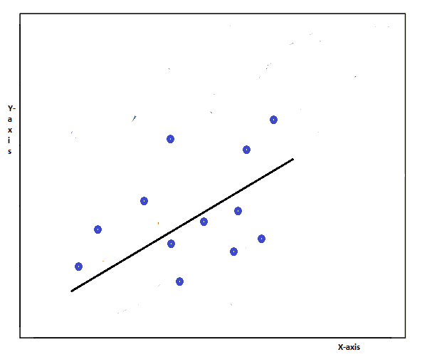
Linear regression is one of the easiest machine learning algorithms. It is a linear approach to modeling the relationship between a dependent variable and an independent variable. The independent variable is called the predictor.
It consists of graphing a line over a set of data points that most closely fits the overall shape of the data. In other words, it shows the changes in a dependent variable on the y-axis to the changes in the independent variable on the x-axis.
The relationship between two variables is called deterministic if one variable can be accurately expressed by the other variable.
In linear regression, the data is modeled using a straight line. It follows the line equation y = mx+c, which you may have already studied in your high school mathematics.
In this equation, y is the dependent variable, x is the independent variable, m is the slope of the line and b is the intercept.
It means that every value of X has a corresponding value of Y in the graph. Linear regression is used with continuous variables. The output of the linear regression equation will be the value of the variable.
For example, we can find the temperature in Fahrenheit if we are given the temperature in degree Celcius. This is easily done by using the equation of the regression line, which is in this case,
F = C * (9/5) + 32
where F is the temperature in Fahrenheit (dependent variable) and C is the temperature in degree Celcius (independent variable).
Now, you may have got a clear idea about what actually linear regression is. Let’s look at the applications of linear regression.
Linear regression can be used to predict trends and future values. It can be used to forecast the impact of changes. It can also be used to predict the strength of the effects that the independent variables have on the dependent variables.
In Python, we have a module called LinearRegression in the scikit learn library that we can use to implement linear regression.
If there is only one independent variable, we call it a simple linear regression. If there is more than one independent variable, then we call it multiple linear regression.
Now, let’s move on to the next supervised learning algorithm.
Logistic Regression
Logistic regression is another type of regression analysis. This algorithm is mostly used when the output or dependent variable is in binary format.
It produces results in a binary format that is used to predict the outcome of a categorical dependent variable. So, the outcome is always categorical or discrete such as 0 or 1, true or false, yes or no, high or low, pass or fail, etc.
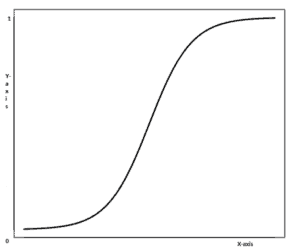
In this, the resulting curve cannot be formulated into a single equation. Since the logistic experiments can only have one of two possible values for each experiment, the points will not be normally distributed about the predicted line.
Hence, we use a logistic. Logistic regression produces a logistic curve, which is limited to values between 0 and 1. This curve is also known as the sigmoid curve or the S-curve.
Logistic regression can be used for classification problems. It is used to estimate the probability that an instance belongs to a particular class.
If the estimated probability is greater than 50%, then the model predicts that the instance belongs to the 1st class, or else it predicts that it does not. This makes it a binary classifier.
Logistic regression is similar to linear regression in computing the weighted sum of the input features. But, instead of outputting the results directly, the logistic regression outputs the logistic of this result.
In Python, we have a module called LogisticRegression in the scikit learn library that we can use to implement logistic regression.
I hope you got a clear idea about logistic regression. Now, it is time to take a look at the next supervised learning algorithm.
K-Nearest Neighbors (KNN algorithm)
The KNN algorithm is one of the simplest algorithms used in machine learning for solving regression and classification problems. This algorithm stores all the available cases and classifies the new data or cases based on a similarity measure.
KNN suggests that if you are similar to your neighbors, then you are one of them. For example, if mango looks most similar to orange, apple, and grapes compared to tiger, cat, and dog, then we can say that mango is more likely to be a fruit rather than an animal.
KNN is used for applications where you are looking for similar items. If the task is to search and find an item similar to the given item, then we can call the search a KNN search.
In KNN, the K denotes the number of nearest neighbors who are “voting” on the test example’s class.
When tested with a new example, KNN looks through the training data and finds the K training examples that are closest to the new example. It then assigns the most common class label (among those K training examples) to the test example.
If the value of K is 1, then test examples are given the same label as the closest example in the training set. If K=3, the labels of the three closest classes are checked and the most common label is assigned, and so on for large values of K.
One commercial application of the K-nearest-neighbors algorithm is the recommendation of products on Amazon or any other shopping website. It is also used in image recognition, text recognition, etc.
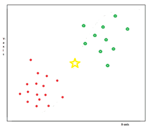
Take a look at this example graph. Here, we have two categories represented by the red circles and the green circles. We have an input point, which is represented by the yellow star-shaped symbol.
We need to find whether this new point belongs to the red category or the green category. This is done by taking the K (for example K=5) nearest neighbors and calculating their distance from the new point.
Based on these calculations, KNN will predict whether this point belongs to the red category or the green category.
The distances can be of different types such as Euclidean distance, Hamming distance, Manhatten distance, Minkowski distance, etc.
I don’t want to scare you with all these words. I just want to let you know that the distance can be calculated in different ways.
Support Vector Machine (SVM algorithm)
Support Vector Machine is a powerful machine learning model used for performing linear or non-linear classification or regression. SVM is specific to supervised learning.
Given a set of training examples, each labeled as belonging to one or the other of two categories, an SVM training algorithm builds a model that assigns new examples to any one of these two categories.
SVM makes use of a hyperplane, which acts as a decision boundary between the various classes. It is mainly used for classification purposes.
It can generate multiple hyperplanes to separate the data into different segments. Each of these segments contains only one kind of data.
SVM classifies any new data depending on what it learned during the training process.
A support vector is a vector that denotes a point in three-dimensional space and it starts from the origin to that point.
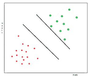
Take a look at this graph. We have two categories, green and red. We want to draw a line to separate these two categories.
We need to get the exact line so that it separates our existing data as well as the future data that comes up. This problem is easily solved by the support vector machine algorithm.
Let’s say we have a line. We need to maximize the margin between the adjacent points on either side of the line. That is how we get the most suitable line which divides the categories.
So, given labeled training data, the SVM algorithm outputs an optimal hyperplane that categorizes new examples. You can see the hyperplanes on the above-given graph.
Now, let’s learn the next algorithm.
Decision Trees
Decision trees are very powerful machine learning algorithms that can perform both classification and regression tasks. They are capable of fitting complex datasets and can even perform multioutput tasks.
A decision tree is a graphical representation of all the possible solutions to a decision based on certain conditions. It starts with a root and then branches out to various solutions, just like a tree.
Decision trees are very easy to read and understand. They are mainly used for classifications. You can see exactly why the classifier made a particular decision.
A decision tree is a decision support tool that uses a tree-like model of decisions and their possible consequences, including chance event outcomes, resource costs, and utility.
If you are a programmer, you already know about conditional statements, right? We write programs to check an if condition and it will do corresponding things when that condition is satisfied. If the condition was not met, then it will check the next condition, and so on.
Decision trees are similar to conditional statements. It works in the same manner until it finds the desired result.
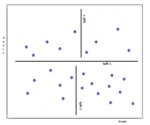
Let’s take a look at this graph. The decision tree algorithm performs various split functions to find the result. These splits are represented by the lines in this graph. A condition check is performed at each of these splits.
For example, at split 1 the algorithm finds that our desired result is located above the split 1 line in this graph. So, it can eliminate the region below that line from consideration.
Similarly, it performs various splits to narrow down the sample space and eventually finds the desired result.
One important advantage of decision trees is that they require very little data preparation. Particularly, they don’t require feature scaling or centering at all.
Python provides modules like DecisionTreeClassifier and DecisionTreeRegressor along with its scikit learn library for easily implementing decision trees.
Random Forests
Random forests or random decision forests are ensemble learning methods for classification, regression, and other tasks. These are made by using many decision tree models.
You can get the idea from the name itself. A collection of trees is called a forest, right? Similarly, a collection of decision trees can be called a Random Forest.
Ensemble learning is the process by which multiple models are strategically generated and combined to solve a particular computational intelligence problem.
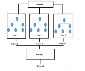
This algorithm operates by constructing multiple numbers of decision trees at training time and outputting the class that is the mode of the classes or mean prediction of the individual trees.
It introduces some extra randomness when growing trees. Unlike decision trees, when splitting a node, the Random Forest algorithm searches for the best feature among a random subset of features. This results in a greater tree diversity which yields an overall better model.
Each decision tree used in this model results in certain outputs. The random forest algorithm combines all these outputs to bring up the final result.
It uses a voting method to produce the correct output from the set of outcomes from the decision trees.
To implement this algorithm in Python, the scikit learn library provides two modules RandomForestClassifier and RandomForestRegressor for classification and regression processes respectively.
Neural Networks
An artificial neural network is a computer system modeled on the human brain and nervous system. These systems learn to perform tasks by considering examples, generally without any prior knowledge of the tasks.
We know how the human brain works, don’t we? Our biological neural networks or our brain learns from the information given by others as well as the information learned by itself. We can also learn from the mistakes that we do.
Similarly, an artificial neural network can also do these functions and learn to do many tasks.
Neural networks are widely used in several real-world applications such as pattern recognition, signal processing, voice recognition, face recognition, self-driving cars, etc.
An artificial neural network consists of a collection of connected units or nodes called artificial neurons. Each connection, like the synapses in a biological brain, can transmit a signal from one artificial neuron to the next one.
An artificial neuron that receives a signal can process it and then signal additional artificial neurons connected to it. ANNs are mainly used to solve complex problems in computer science.
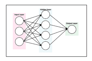
Take a look at this diagram of a basic neural network. It mainly consists of three layers. An input layer, an output layer, and a hidden layer. The layers are made of one or more nodes. A node is just a place where computation happens.
The hidden layers can be one or more. A neural network with multiple hidden layers is called a deep neural network. These neural networks help us to cluster and classify complex datasets.
We can give a dataset as input to the neural network. It will process the data by using various machine learning or deep learning algorithms. The patterns they recognize are numerical, contained in vectors, into which all real-world data like images must be translated.
Conclusion
Supervised learning is one of the important types of machine learning tasks. It can be done by using various algorithms.
In this article, we have discussed 7 important supervised algorithms. Apart from these, there are many other algorithms as well. New algorithms are being developed day by day.
If you want to learn more about supervised learning algorithms, check out this scholarly article.
I have written an article on the advantages as well as the disadvantages of using supervised machine learning. You can check that out by clicking here.
If you have any doubts or queries, feel free to ask them in the comments. If this article was helpful, do share it on social media.
Recent Posts
Modular programming is a software design technique that emphasizes separating the functionality of a program into independent, interchangeable modules. In this tutorial, let's understand what modular...
While Flask provides the essentials to get a web application up and running, it doesn't force anything upon the developer. This means that many features aren't included in the core framework....
